Big O notation is primarily used to describe the upper bound or worst-case time complexity of an algorithm. It provides an estimation of how an algorithm's runtime will grow as the input size increases to its largest possible value. In this article, I will go over what Big O is, its history, how it is used, and some examples of the different Big O time complexities that you commonly see. This will be a very long article, so you may have to come back to it several times, but don't worry, I'm going to try to explain things to you as simply as I can.

History

Let us take a brief look at the history that would lead to the use of Big O notation. Paul Bachmann and Edmund Landau, German mathematicians, developed a family of notations, collectively called Bachmann-Landau notation. This was used for describing the asymptotic behavior of functions. Big O also happened to be one of those notations.

In the early 20th century, Electronic computers were becoming a reality and as they evolved, the need for computer scientists to build and optimize algorithms for various problems became more important. Early computer scientists were often mathematicians and engineers so they were tasked with creating algorithms for tasks such as numerical computation, data processing, and cryptography. Eventually, computer scientists needed a systematic way to analyze and describe the performance of algorithms. This would lead to the exploration of math tools and notations for expressing time complexity.

Computer scientists and mathematicians would use various notations such as Landau notation to describe the growth rates of functions until Donald Knuth wrote "The Art of Computer Programming" which was published in 1968. Big O gained prominence because of its simplicity and expressiveness as it provided a straightforward way to describe how the runtime of an algorithm scales with input size. Knuth's work helped codify the usage of Big O and its adoption in Computer Science.

The reason Knuth's work had an impact on the standardization of Big O notation as a measure of time complexity was due to the clarity and comprehensive analysis of Big O notation.

Rate of Change

When measuring the time complexity of an algorithm, it is not measured by seconds but by rate of change.

Rate of change - the speed at which a variable changes over time. The acceleration or deceleration of changes, not the magnitude of individual changes.

$$R = \Delta y / \Delta x$$

Rate = change in y / change in x

It is often used when speaking about momentum, i.e. price returns and identifying momentum in trends in Finance, distance vs. time in Physics, population growth in Biology, derivatives in Calculus, and Sine Function in Trigonometry.

Imagine you have a dictionary with 100 pages. You are looking for the word "lethargic".

• Method 1: You start at the beginning of the dictionary and search each page until you find the word. This will take you a long time because you have to search through each page after the other until you find the word. The rate of change is low.

• Method 2: You open the dictionary to the middle page, which is page 50. You then look at the first half of the dictionary (pages 1-50) and the second half of the dictionary (pages 51-100). You know that the word "lethargic" is not on pages 51-100, so you only have to search through pages 1-50. This will take you much less time than method 1. The rate of change is high.

So, the rate of change in the search process is high when you use a method that allows you to quickly narrow down the search space. The rate of change is low when you use a method that requires you to search through a large number of items.

Linear Search vs. Binary Search

A linear search is much slower than a binary search. Why? Because a linear search is accessing each element of an array until the target is found whereas a binary search is splitting the array in half each time until the target is found.

// O(n)
public int linearSearch(int[] arr, int target) {
    for(int i = 0; i < arr.length - 1; i++) {
        if(arr[i] == target) return i;
    }

    return -1;
}

// O(log n)
public int binarySearch(int[] arr, int target) {
    int low = 0, high = arr.length - 1;

    while(low <= high) {
        int middle = (low + high) / 2;

        if(arr[middle] == target) {
            return middle;
        } else if(arr[middle] < target) {
            left = middle + 1;            
        } else {
            right = middle - 1;
        }
    }

    return -1;
}

The Common Big O Notation Time Complexities

You were just introduced to two complexities, O(n) and O(log n). Now let's look at the other ones in more detail.

O(1) - Constant Time - Extremely Fast

The algorithm's runtime is constant and does not depend on the input size. In this example, all that is being done is accessing the area and returning it. No changes have been made. The simplest example is accessing and returning an element in an array. No extra steps are required. It takes the same amount of time no matter the size of the array since you can directly jump to the memory location of the desired index.

public int getElementAtIndex(int[] inputArray, int index) {
    return inputArray[index];
}

More examples:

1. Checking if a Queue is Empty

2. Finding the First Element in a Linked List

3. Hash Table Lookup

4. Incrementing a Counter

5. Checking if a Set Contains an Element

O(log n) - Logarithmic Time - Very Fast

The algorithm's runtime grows logarithmically with the input size. This time complexity is considered very efficient especially when the input size is large. The time it takes to run the algorithm does not grow as quickly as the input size. Binary search is one example.

More Examples

1. Finding an Element in a Balanced Binary Search Tree

2. Searching in a Phone Book with Dividing Sections

3. Merge Sort(requires backtracking and recursion)

4. Divide and Conquer Algorithms

5. Binary Heap Operations

O(n) - Linear time - Mid

The notation O(n) represents linear time complexity, where the runtime of an algorithm increases linearly with the size of the input. In the previous section, Linear search vs. Binary search, linear search is O(n) because it keeps iterating through the array, accessing each element until a target is found. Though this doesn't require any extra steps and is very simple to implement, this could be very slow, especially the bigger the array gets. Imagine searching each element in an array one by one when the length of the array is 1000, 10,000, 100,000+.

More Examples:

1. Copying Elements from One Array to Another

2. Linear Search in Linked List

3. Finding Maximum/Minimum in an Array

4. Calculating the Sum or Average of Array Elements

5. Iterating Through a Graph

O(n log n) - Linearithmic time - A little on the slow side

The algorithm's runtime grows logarithmically (n times the logarithm of n) with the input size. A merge sort runs at O(n log n) because it divides the input array into smaller subarrays and then merges them together in a sorted manner. The combination of division and merging gives Merge Sort a time complexity of O(n log n).

public int[] sortArray(int[] nums) {

        mergeSort(nums, 0, nums.length - 1);

        return nums;
    }

    //O(log n)
   public void mergeSort(int[] nums, int left, int right) {
        if(left < right) {
            int middle = (left + right) / 2;
            mergeSort(nums, left, middle);
            mergeSort(nums, middle + 1, right);
            merge(nums, left, middle, right);
        }
   }

   //O(n)
    public void merge(int[] nums, int left, int middle, int right) {
        int n1 = middle - left + 1;
        int n2 = right - middle;

        int[] L = new int[n1];
        int[] M = new int[n2];

        for(int i = 0; i < n1; i++) {
            L[i] = nums[left + i];
        }

        for(int i = 0; i < n2; i++) {
            M[i] = nums[middle + 1 + i];
        }

        int i = 0, j = 0, k = left;

        while(i < n1 && j < n2) {
            if(L[i] <= M[j]) {
                nums[k] = L[i];
                i++;
            } else {
                nums[k] = M[j];
                j++;
            }
            k++;
        }

        while(i < n1) {
            nums[k] = L[i];
            i++;
            k++;
        }

        while(j < n2) {
            nums[k] = M[j];
            j++;
            k++;
        }
    }

More Examples:

1. Heap Sort

2. Balanced Binary Search Tree Operations

3. Divide and Conquer Algorithms (Certain Cases)

4. Fast Fourier Transform (FFT)

5. Merge-Based Divide and Conquer Algorithms

6. Distributed Algorithms

O(n^2) - Quadratic time - Slow

The algorithm's running time grows in about the size of the input data. This time complexity often occurs in algorithms that involve nested loops. If you have two nested loops where each loop iterates n times, the total number of iterations will be n * n.

O(n^2) algorithms are considered inefficient for large input sizes because the running time grows quickly as the input size increases.

Bubble Sort: Bubble sort is an example of O(n^2) because it requires using a nested for loop. It repeatedly compares adjacent elements in the input array and swaps them if they are in the wrong order. The outer loop iterates over the array from 0 to n-1. The inner loop iterates over the array from 0 to n-i-1.

public static void bubbleSort(int[] array) {
  int n = array.length;

  for (int i = 0; i < n - 1; i++) {
    for (int j = 0; j < n - i - 1; j++) {
      if (array[j] > array[j + 1]) {
        int temp = array[j];
        array[j] = array[j + 1];
        array[j + 1] = temp;
      }
    }
  }
}

More Examples:

1. Insertion Sort

2. Selection Sort

3. Brute Force Algorithms

4. Checking for Duplicates

5. Some Graph Problems

O(2^n) - Exponential time - Very Slow

The algorithm's runtime grows exponentially with the input size. Algorithms with this time complexity are considered inefficient, especially when the input size is large. The time it takes to run the algorithm grows very quickly as the input size grows.

Recursive Fibonacci Calculation: The naive way of calculating Fibonacci numbers using recursion can result in O(2^n) time complexity due to redundant calculations.

public static int fibonacci(int n) {
  // Base cases.
  if (n == 0) {
    return 0;
  } else if (n == 1) {
    return 1;
  }

  // Recursive case.
  return fibonacci(n - 1) + fibonacci(n - 2);
}

More Examples:

1. Subset Sum Problem

2. Recursive Maze Solving

3. Generation of Power Sets

4. Recursive Tree Traversal

5. Subset Generation Using Bitmasks

6. Exact Cover Problem

It's important to note that algorithms with exponential time complexity become extremely slow as the input size increases, even for relatively small inputs. They're generally not practical for real-world applications unless the input size is very small. In many cases, efforts are made to find more efficient algorithms that can solve these problems in polynomial or linear time complexity.

O(n!) - Factorial time - Extremely Slow

The algorithm's runtime grows factorially with the input size. An example of that would be permutations, which are one of several possible variations in which a set of numbers can be ordered or arranged.

Permutations and Combinations: When generating all possible permutations or combinations of a set of elements, the number of arrangements or selections grows factorially with the number of elements.

import java.util.ArrayList;
import java.util.List;

public class Permutations {
    public List<List<Integer>> permute(int[] nums) {
        List<List<Integer>> result = new ArrayList<>();
        backtrack(nums, 0, result);
        return result;
    }

    private void backtrack(int[] nums, int start, List<List<Integer>> result) {
        if (start == nums.length) {
            // Convert the current permutation array to a list and add it to the result
            List<Integer> permutation = new ArrayList<>();
            for (int num : nums) {
                permutation.add(num);
            }
            result.add(permutation);
        }

        for (int i = start; i < nums.length; i++) {
            // Swap elements at indices start and i
            swap(nums, start, i);
            // Recursively generate permutations
            backtrack(nums, start + 1, result);
            // Undo the swap for backtracking
            swap(nums, start, i);
        }
    }

    private void swap(int[] nums, int i, int j) {
        int temp = nums[i];
        nums[i] = nums[j];
        nums[j] = temp;
    }

    public static void main(String[] args) {
        int[] nums = {1, 2, 3};
        Permutations permutations = new Permutations();
        List<List<Integer>> result = permutations.permute(nums);
        for (List<Integer> permutation : result) {
            System.out.println(permutation);
        }
    }
}

More Examples

1. Traveling Salesman Problem

2. Brute Force Cryptanalysis

3. Recursive Algorithms without Memoization

4. Exact String Matching using Brute Force

5. Generating All Possible Subsets

6. Tiling Problems

7. Solving the Eight Queens Puzzle

Conclusion

In conclusion, Big O notation provides a vital framework for understanding and analyzing the efficiency of algorithms in terms of their time complexity. It offers a standardized way to express how an algorithm's runtime scales with input size, allowing us to make informed decisions about algorithm selection. We've explored the history and development of Big O notation, from its origins in the work of mathematicians like Bachmann and Landau to its widespread adoption in computer science, thanks to Donald Knuth's pioneering efforts.

We've also delved into different time complexities, from O(1) representing constant time to O(n!) indicating factorial time. The choice of algorithm and its time complexity can significantly impact performance, as demonstrated by the difference between linear and binary search methods.

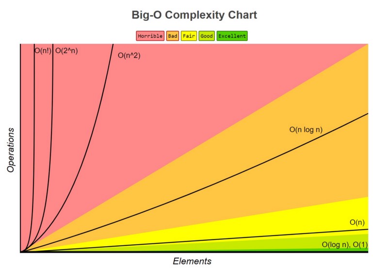
Finally, we've seen various common Big O notation rates in action, ranging from the highly efficient O(1) and O(log n) to the less efficient O(n) and O(n log n), all the way to the slow O(n^2), O(2^n), and O(n!) algorithms. Understanding these complexities is crucial when designing efficient algorithms for solving real-world problems. So, whether you're searching for the quickest path, sorting a list, or optimizing a computation, Big O notation equips you with the tools to make informed decisions about algorithm selection and performance optimization.

If you have any questions, please leave them in the comment section or if you're shy, you can DM me on Twitter/X. Happy coding!